YIG-Tuned Filters: Selection and Specification

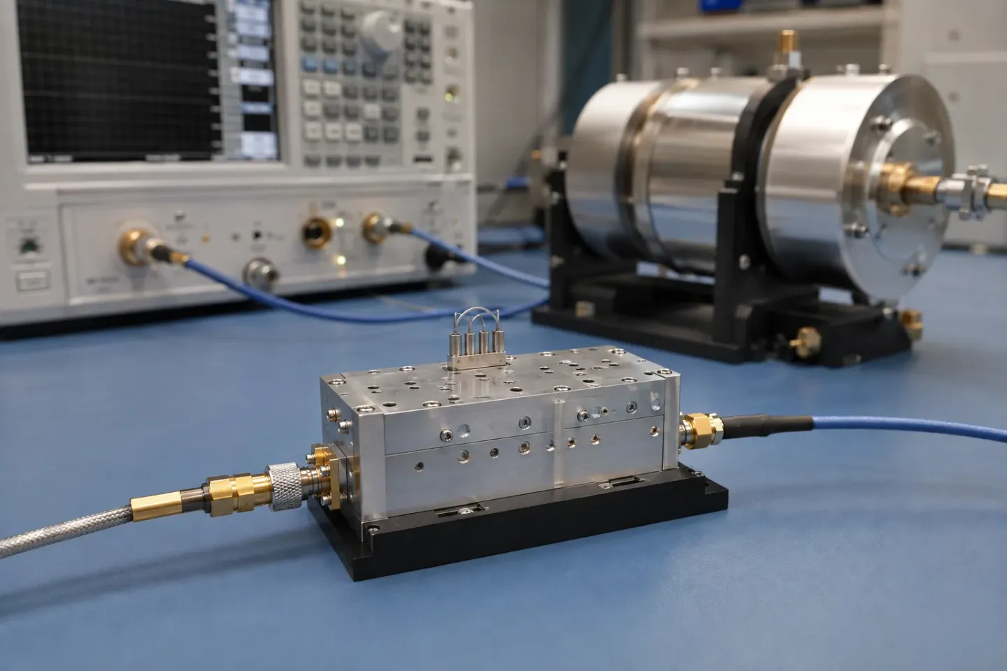
A YIG-tuned filter is a microwave filter whose centre frequency is set by a magnetic field rather than by a machined dimension. One or more polished YIG spheres sit in a common electromagnet. Small coupling loops transfer energy into and out of each sphere only at the resonant frequency of that field. Change the coil current and the passband — or the notch — moves with it, across an octave or more, at a width measured in tens of megahertz rather than as a percentage of centre.

That combination is why the components that sit in front of a broadband mixer are so often YIG filters. A cavity can be cleaner and lower-loss at one frequency. It cannot follow the LO.

Where it sits in the chain

In a receiver the filter is usually a tracking preselector: it sits after the antenna (and often after a limiter and LNA) and before the mixer, and it moves with the local oscillator. Its job is to pass the wanted RF and reject everything that would mix to the same IF — first of all the image, 2 × IF away. After the mixer it is too late; the image and the wanted signal are the same frequency.

In test equipment the same part is a tunable bandpass or band-reject in front of a detector or a spectrum analyser. The specification language does not change. The time budget does: a sweeper that steps the LO and the preselector together spends settling time twice.

How it works

The resonator is the same ferrimagnetic sphere used in a YIG oscillator. The difference is the coupling.

In a bandpass filter the input and output loops are set at 90° so that energy cannot cross except through the resonating spheres. Closer loop-to-sphere spacing widens the 3 dB bandwidth and raises insertion loss. More spheres, carefully aligned, do the same and also steepen the skirt.

In a band-reject filter a single loop per sphere lies along the transmission path. Off resonance the loop is just line; on resonance it couples to the sphere and reflects. Rejection width is opened the same way as passband width: more spheres, tighter coupling. Standard 40 dB notch widths for this class sit around 15 to 70 MHz.

Both types follow coil current, not voltage. The driver is half the specification, for the same reason it is on a YTO.

Key specifications

Parameter	What it means	What it constrains
Tuning range	Span over which the magnet can place the band	Whether one filter covers the receiver, or you need several
3 dB bandwidth	Absolute width of the passband or notch, at a stated frequency	Channel width versus interferer rejection
Stage count	Number of spheres in the coupling path	Skirt steepness and insertion loss together
Insertion loss	Passband loss at the tuned centre	System noise figure, if the filter sits before the LNA — or after it, the recovery you still need
Off-resonance isolation	Rejection away from the tuned band	Image rejection and blocking
Limiting level	Input power at which the sphere saturates	Whether a large signal collapses the filter
Settling time	Time to sit inside a frequency tolerance after a step	Sweep or hop rate, usually added to the LO’s
Passband VSWR / ripple	Match and flatness across the 3 dB width	Whether the LNA or mixer sees a stable load as you tune

Meanings are general to the device class. For values, work from the specific part’s datasheet — stage count, band and grade move every number.

For the figures we can attribute, the manufacturer’s published description gives standard bandpass 3 dB bandwidths of 15 to 40 MHz at 2 GHz and 20 to 50 MHz at 18 GHz, and standard band-reject parts with a 40 dB rejection bandwidth of 15 to 70 MHz.

Stage count, insertion loss by stage, selectivity in dB per octave and temperature grades vary widely by band and product line, and the primary documents carrying those tables are published as scanned PDFs we could not read. We therefore state the relationships rather than numbers: more stages steepen the skirt and add insertion loss, and that is one trade rather than two. Work the actual values from the datasheet of the specific part.

Bandwidth is not quite constant

A selling point of YIG filters is a constant absolute bandwidth — tens of megahertz at 2 GHz and still tens of megahertz at 18 GHz, where a percentage-bandwidth cavity would have opened by a factor of nine. The published correction is that the 3 dB width still expands at about 20% per octave (the manufacturer’s own example is 30 MHz at 2 GHz becoming 50 MHz at 18 GHz). Specify the width at the frequencies you will use, not only at the bottom of the band.

The sphere also has a limiting level, typically 0 to +10 dBm. That is not a damage spec in the usual sense; it is the power at which the resonator stops coupling the way the datasheet assumed.

Against the alternatives

Criterion	YIG-tuned filter	Cavity filter	Switched filter bank
Tuning	Electrical, octave or more	Mechanical, or none	Discrete bands only
Bandwidth vs frequency	Roughly constant absolute width	Percentage of a fixed centre	Whatever each cavity was cut for
Insertion loss	Rises with stage count	Lower than a YIG filter	Cavity-like, plus switch loss
Selectivity	Set by stage count; good, not cavity-Q	Higher Q than a YIG resonator	Per-band, cavity-like
Settling	Milliseconds (coil)	None, or mechanical	Switch time
Power handling	Limited by sphere saturation	High; radar and SATCOM use it	High per path
Size and power	Magnet dominates; coil current continuous	Machined metal; no coil	Several cavities plus switches
Typical use	Tracking preselector, analyser	Fixed channel, high power	A short list of bands

The pattern matches the oscillator comparison: YIG buys a moving, constant-width band and pays in loss, speed and size. When the band does not move, a cavity is the better filter. When you need both low loss and several discrete bands, a switched bank is the honest alternative — not a “faster YIG”.

Application matrix

Application	What dominates the choice	Where a YIG filter struggles
Spectrum / signal analyser preselector	Multi-octave tune at a constant absolute width	Sweep rate; insertion loss ahead of the converter
EW / SIGINT receiver	Tracking the LO across the threat band	Hop speed; limiting on large signals
Spectrum monitoring front end	Coverage plus a tracking pair with the LO	Combined settling of filter and oscillator
Radar front end	Image and blocker rejection that can move	Pulse-to-pulse agility; power handling
ATE / bench filtering	A single tunable bandpass or notch	Cost and coil power versus a drawer of cavities
SATCOM channel filter	Almost never YIG	Loss, size and a band that does not move

Qualitative. Every row is a judgement about which parameter binds first, not a vendor recommendation.

A monitoring or EW front end usually pairs the filter with a YIG-tuned oscillator. Both are magnetically tuned, so both settle in milliseconds, and those times add. A preselector’s insertion loss lands on the system noise figure if it sits before the first gain stage, and still costs you recovered gain if it sits after — so the isolation it buys has to be worth that.

Selection criteria

Advantages and limitations

Advantages. Multi-octave electrical tuning from one device. Roughly constant absolute bandwidth. Linear frequency-versus-current. Stage count as a single, understandable selectivity control. The only practical tracking preselector for a wideband receiver.

Limitations. Millisecond settling. Continuous coil power. Insertion loss that grows with the selectivity you asked for. Sphere limiting at modest power. Magnetic sensitivity. A package set by the magnet. A 3 dB width that still creeps ~20% per octave.

Typical applications

Wideband receivers and spectrum analysers, as the tracking preselector in front of the first mixer. Electronic-warfare and spectrum-monitoring front ends, paired with a YTO. Bench and ATE filtering where one tunable bandpass or notch replaces a drawer of cavities. Radar, when the front end must move and the pulse timing can afford the settle — see radar RF components.

Buying and lifecycle

• Specify stages against an offset, not against a catalogue habit. Four stages you do not need are insertion loss you still pay.
• Ask at which frequency the 3 dB width was measured. The ~20% per octave creep makes a single number incomplete.
• Ask what driver the accuracy figure was taken with. Current noise on the coil is frequency modulation of the passband.
• Check limiting against the largest signal the antenna can present, including after the LNA if the filter sits there.
• Plan calibration with the LO. A tracking pair that is calibrated apart will not track in the box.

Obsolescence on a low-volume magnetic part is the same problem as on a YTO; the general discipline is in sourcing and quality.

Testing and integration notes

• Measure isolation at the image frequency of the actual IF plan, not only at a convenient offset on the bench.
• Verify settling with the same step size the LO will take. A full-band figure does not describe a 50 MHz correction.
• Sweep insertion loss and VSWR across the tune; a filter that is pretty at centre and ugly at the band edge is a common surprise.
• Confirm the limiting level with the real source, not a swept synthesizer parked at −20 dBm.
• Check magnetic clearance before the enclosure is fixed. The control variable is a field.

Related guides

• What is YIG — the material and why a sphere tunes at all
• YIG filter vs cavity filter — the decision this pillar assumes
• RF, IF and LO explained — why the image is 2 × IF away
• YIG oscillators — the usual tracking partner
• Understanding phase noise — reciprocal mixing is why the preselector exists
• Radar RF components — how the same parts are constrained in a radar

Set a tracking budget, not two independent specifications

The common YIG-filter application is a receiver whose LO and preselector move together. It is tempting to specify oscillator tuning accuracy on one sheet and filter tuning accuracy on another, then expect the pair to work after installation. The meaningful quantity is their relative error. The filter has to remain centred on the wanted RF while its reject band stays useful at the image or blocker location. Two individually accurate current tables can still drift apart after temperature, cable resistance or a different approach direction are introduced.

Begin by deciding what the filter must pass. Include the wanted signal bandwidth, modulation shoulders, frequency error, calibration error and any required margin. Then state the rejection required at the calculated image and known blocker offsets. This creates an allowed tracking error across the band. A wide passband is more forgiving of tracking but sacrifices rejection; a narrow passband protects the mixer but makes error and settling visible. The right budget comes from the receiver plan, not from a favourite stage count.

Command sequencing belongs in that budget. If a YTO moves to a new frequency and the filter follows, define when each current is updated, how long each is allowed to settle and which indication declares the receiver ready. A full-span calibration is useful, but operational tests must also use small corrections and reversals, because magnetic history can affect both devices. The corresponding source behaviour is described in how YIG oscillators work.

Noise and loss remain separate constraints. A quiet LO does not compensate for a preselector that lets a strong blocker reach the mixer, while a narrow filter does not improve a noisy LO at an in-band offset. Conversely, every dB of filter loss ahead of the first gain stage costs sensitivity. Test the complete chain at the intended RF points with desired and blocker signals, then compare the result with the phase-noise requirement rather than assigning all degradation to one part.

For maintainable systems, store the filter calibration, driver revision, temperature reference and acceptance sweep with the serial number. A replacement filter may match the catalogue range yet require its own table; traceable test evidence is what turns an interchangeable-looking component into a reliable tracking pair.